3-7 Sequential Sorting Algorithms

In 3-5 we learned two different approaches to searching for a given key in a set of data. Although the linear and binary searches achieve the same end result we saw that they are quite different in terms of design and performance. Moreover, they can each be implemented using either loops or recursion.

Now we’ll turn our attention to sorting data. Sorting means to arrange a group of items into a particular order such as ascending or descending. Sorting is a classic problem in computer science and there are many sorting algorithms! Some sorting algorithms lend themselves to iteration (we call these sequential sorts), while other are more naturally recursive (we call these recursive sorts). Today we’ll discuss sequential sorting algorithms and next time we’ll tackle recursive sorts.

Bubble Sort v1.0

The bubble sort is a sequential sorting algorithm, and traditionally the first one that students of computer science study. We’ll cover 3 progressively more efficient versions of the algorithm to illustrate how minor code improvements can have major impacts on performance.

The basic (version 1.0) bubble sort works like this:

Let # of passes required = array.length – 1

Do this # of passes times:
- Compare each pair of adjacent elements in the array from first to last. If two elements are in the wrong order, exchange (or “swap”) them!

Below is an illustration of this sorting process with 6 integers. The “C=” refers to the number of comparisons made during the pass through the array, and “E=” refers to the number of exchanges (swaps) made during each pass.

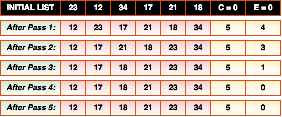
Notice that during each pass through the array exactly 5 comparisons are made since there are 5 pairs of adjacent elements in a 6-element array. In early passes, quite a few exchanges are made, but this decreases in later passes as the data becomes more sorted.

Here is the code for the v1.0 bubble sort (where data is an array of integers):

for ( int pass=1; pass < data.length; pass++ ) {
    for ( int index=0; index < data.length-1; index++ ) {
        // Compare adjacent elements and swap them if necessary
        if ( data[index] > data[index+1] ) {  
            swap( index, index+1 );
        }
    }
}

for ( int pass=1; pass < data.length; pass++ ) {

for ( int index=0; index < data.length-1; index++ ) {

// Compare adjacent elements and swap them if necessary

if ( data[index] > data[index+1] ) {

swap( index, index+1 );

}

You’ll notice that we have 2 nested loops here – meaning that bubble sort is an O(n²) algorithm. It’s simple to code and not bad performance-wise for small data sets but we would not expect it to be very effective for large data sets.

I have created a helper method called swap() that exchanges two elements in the data array. You will recall from 2-9 (Inverting a Fraction) why a temporary variable is needed to swap two array elements.

// helper method to swap values in two data elements
private void swap( int first, int second ) {
    int temporary = data[ first ];  
    data[ first ] = data[ second ]; 
    data[ second ] = temporary;     
}

// helper method to swap values in two data elements

private void swap( int first, int second ) {

int temporary = data[ first ];

data[ first ] = data[ second ];

data[ second ] = temporary;

}

Bubble Sort v2.0

Not bad, but we can double the efficiency! Consider the following diagram:

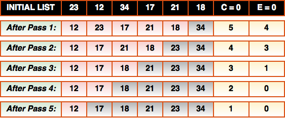
Notice that after each pass through the array, the largest element gets moved (or “bubbled”) to its proper place at the end of the array (these are the elements I’ve greyed out). In other words, after the first pass we can be sure that the largest item (34) is the last element in the array. And, after the second pass, we can be sure that the second largest item (23) in is in second last element of the array etc.. This means that we should be able to do one less comparison on each pass through the data.

Despite this fact, the v1.0 bubble sort code above will compare these elements anyway even though they are already in correct order. The solution to this is very simple: we just do one less comparison on each pass through the array as shown in this code:

for ( int pass=1; pass < data.length; pass++ ) {
    for ( int index=0; index < data.length-pass; index++ ) {
        // Compare adjacent elements and swap them if necessary
        if ( data[index] > data[index+1] ) {  
            swap( index, index+1 );
        }
    }
}

for ( int pass=1; pass < data.length; pass++ ) {

for ( int index=0; index < data.length-pass; index++ ) {

// Compare adjacent elements and swap them if necessary

if ( data[index] > data[index+1] ) {

swap( index, index+1 );

}

Notice in the inner loop continuation condition (line 2) that index is compared to data.length-pass. This ensures that on pass 1 of the outer loop, the inner loop will perform 5 (i.e., data.length of 6 – pass of 1) comparisons. On pass 2 of the outer loop, the inner loop will perform 4 (i.e., data.length of 6 – pass of 2) comparisons, and so on. This tiny change has cut the number of comparisons required by the bubble sort in half! Even with this 50% performance improvement, the bubble sort is still an O(n²) algorithm.

Bubble Sort v3.0

But can we do even better? Yes! If you notice in the previous diagram, exchanges are happening at every pass through the array except passes 4 and 5. This means that after pass 4 we can determine that the array must be sorted and any further passes are unnecessary.

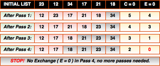
We can use this to our advantage! If we keep track of whether an exchange was made during each pass through the array then we can stop sorting whenever we complete a pass where no exchanges needed to be made. Here’s the most optimal (v3.0) bubble sort code:

boolean exchangeMade = true;

for ( int pass=1; pass < data.length && exchangeMade; pass++ ) {
    exchangeMade = false;
    for ( int index=0; index < data.length-pass; index++ ) {
        // Compare adjacent elements and swap them if necessary
        if ( data[index] > data[index+1] ) {  
            swap( index, index+1 );
            exchangeMade = true;
        }
    }
}

boolean exchangeMade = true;

for ( int pass=1; pass < data.length && exchangeMade; pass++ ) {

exchangeMade = false;

for ( int index=0; index < data.length-pass; index++ ) {

// Compare adjacent elements and swap them if necessary

if ( data[index] > data[index+1] ) {

swap( index, index+1 );

exchangeMade = true;

}

Putting It All Together

Ok, let’s put these 3 variations together into a BubbleSort class:

import java.util.Random;
import java.util.Arrays;

public class BubbleSort {
    private int[] data;
    public static final int RANDOM = 0;
    public static final int ASCENDING = 1;
    public static final int DESCENDING = 2;
    
    // create array of given size and fill with random integers
    public BubbleSort( int size ) {
        this( size, RANDOM );
    }
    
    // create array of given size and fill with integers in a specified order
    public BubbleSort( int size, int order ) {
        Random generator = new Random();
        data = new int[ size ];
        
        for ( int i = 0; i < size; i++ ) {
            data[ i ] = 100 + generator.nextInt(900);
            // BETTER: data[ i ] = generator.nextInt();
        }
        
        if (order == RANDOM)
            return;
        else {
            Arrays.sort(data);
            if (order == ASCENDING)
                return;
            else if (order == DESCENDING) {
                for(int i=0; i < data.length / 2; i++) {
                    // swap the elements
                    swap( i, data.length-(i+1) );
                }
            }
        }
    }
    
    // sort array using bubble sort - level 1
    public void bubbleSortv1() {
        for ( int pass=1; pass < data.length; pass++ ) {
            for ( int index=0; index < data.length-1; index++ ) {
                // Compare adjacent elements and swap them if necessary
                if ( data[index] > data[index+1] ) {  
                    swap( index, index+1 );
                }
            }
            // Output for testing purposes only, REMOVE if timing the algorithm!
            System.out.printf( "After pass #%2d, array is: %s", pass, this );
        } 
    }
    
    // sort array using bubble sort - level 2
    public void bubbleSortv2()
    {
        for ( int pass=1; pass < data.length; pass++ ) {
            for ( int index=0; index < data.length-pass; index++ ) {
                // Compare adjacent elements and swap them if necessary
                if ( data[index] > data[index+1] ) {  
                    swap( index, index+1 );
                }
            }
            // Output for testing purposes only, REMOVE if timing the algorithm!
            System.out.printf( "After pass #%2d, array is: %s", pass, this );
        } 
    }
    
    // sort array using bubble sort - level 3
    public void bubbleSortv3() {
        boolean exchangeMade = true;
        
        for ( int pass=1; pass < data.length && exchangeMade; pass++ ) {
            exchangeMade = false;
            for ( int index=0; index < data.length-pass; index++ ) {
                // Compare adjacent elements and swap them if necessary
                if ( data[index] > data[index+1] ) {  
                    swap( index, index+1 );
                    exchangeMade = true;
                }
            }
            // Output for testing purposes only, REMOVE if timing the algorithm!
            System.out.printf( "After pass #%2d, array is: %s", pass, this );
        }
    }
    
    // helper method to swap values in two data elements
    private void swap( int first, int second ) {
        int temporary = data[ first ];  
        data[ first ] = data[ second ]; 
        data[ second ] = temporary;     
    } 
    
    // Return string representing all elements in array
    public String toString() {
        return Arrays.toString( data ) + "\n";
    } 
}

import java.util.Random;

import java.util.Arrays;

public class BubbleSort {

private int[] data;

public static final int RANDOM = 0;

public static final int ASCENDING = 1;

public static final int DESCENDING = 2;

// create array of given size and fill with random integers

public BubbleSort( int size ) {

this( size, RANDOM );

}

// create array of given size and fill with integers in a specified order

public BubbleSort( int size, int order ) {

Random generator = new Random();

data = new int[ size ];

for ( int i = 0; i < size; i++ ) {

data[ i ] = 100 + generator.nextInt(900);

// BETTER: data[ i ] = generator.nextInt();

}

if (order == RANDOM)

return;

else {

Arrays.sort(data);

if (order == ASCENDING)

return;

else if (order == DESCENDING) {

for(int i=0; i < data.length / 2; i++) {

// swap the elements

swap( i, data.length-(i+1) );

}

// sort array using bubble sort - level 1

public void bubbleSortv1() {

for ( int pass=1; pass < data.length; pass++ ) {

for ( int index=0; index < data.length-1; index++ ) {

// Compare adjacent elements and swap them if necessary

if ( data[index] > data[index+1] ) {

swap( index, index+1 );

}

// Output for testing purposes only, REMOVE if timing the algorithm!

System.out.printf( "After pass #%2d, array is: %s", pass, this );

}

// sort array using bubble sort - level 2

public void bubbleSortv2()

{

for ( int pass=1; pass < data.length; pass++ ) {

for ( int index=0; index < data.length-pass; index++ ) {

// Compare adjacent elements and swap them if necessary

if ( data[index] > data[index+1] ) {

swap( index, index+1 );

}

// Output for testing purposes only, REMOVE if timing the algorithm!

System.out.printf( "After pass #%2d, array is: %s", pass, this );

}

// sort array using bubble sort - level 3

public void bubbleSortv3() {

boolean exchangeMade = true;

for ( int pass=1; pass < data.length && exchangeMade; pass++ ) {

exchangeMade = false;

for ( int index=0; index < data.length-pass; index++ ) {

// Compare adjacent elements and swap them if necessary

if ( data[index] > data[index+1] ) {

swap( index, index+1 );

exchangeMade = true;

}

// Output for testing purposes only, REMOVE if timing the algorithm!

System.out.printf( "After pass #%2d, array is: %s", pass, this );

}

// helper method to swap values in two data elements

private void swap( int first, int second ) {

int temporary = data[ first ];

data[ first ] = data[ second ];

data[ second ] = temporary;

}

// Return string representing all elements in array

public String toString() {

return Arrays.toString( data ) + "\n";

}

In today’s exercises you will be implementing another common sequential sorting algorithm. Please pay close attention to how the code above is structured and follow a similar model for your own code.

Line 5 encapsulates the data array, just as we did with our LinearSearch and BinarySearch classes earlier. Lines 6 to 8 provide public constants used to indicate the starting order for the data array (before any bubble sorting takes place). These constants are used in the 2 overloaded constructors.

The first constructor only requires the caller to specify how many integers they would like in the array, and defaults to RANDOM initial order. The second constructor accepts a size, but also allows the caller to control the initial order of the elements in the data array. The RANDOM constant ensures that the data is in completely random order, ASCENDING uses the Arrays.sort() method to put the elements in ascending order, and DESCENDING puts the elements into descending order. It may seem odd to use the Arrays.sort() method in our BubbleSort class, but the point is to allow us to control the starting order of our data so that we can test our bubble sort algorithm against different data sets. It turns out that Arrays.sort() uses a sorting algorithm called the Quick Sort for arrays of primitive types – we’ll learn about this algorithm next time.

After the constructors, we have our methods for the three bubble sort variations, followed by a swap() helper method that is shared by all three, and a toString() method so that we can get a String representation of the elements in our data array. Notice on lines 50, 65, and 83 I am using the toString() method to display the contents of the data array after each sorting pass. These three lines are for testing/demonstration purposes only, one would definitely remove them in a final product.

Here is a test class, demonstrating our bubble sort v3.0 method:

public class BubbleSortTest
{
   public static void main( String[] args ) {
      // create object to perform bubble sort
      BubbleSort sortArray = new BubbleSort( 10, BubbleSort.RANDOM );
      
      System.out.println( "UNSORTED ARRAY: " + sortArray );
      sortArray.bubbleSortv3();
      System.out.println( "\nSORTED ARRAY: "  + sortArray);
   } 
}

public class BubbleSortTest

{

public static void main( String[] args ) {

// create object to perform bubble sort

BubbleSort sortArray = new BubbleSort( 10, BubbleSort.RANDOM );

System.out.println( "UNSORTED ARRAY: " + sortArray );

sortArray.bubbleSortv3();

System.out.println( "\nSORTED ARRAY: " + sortArray);

}

UNSORTED ARRAY: [201, 370, 382, 872, 582, 107, 415, 493, 930, 390]
After pass # 1, array is: [201, 370, 382, 582, 107, 415, 493, 872, 390, 930]
After pass # 2, array is: [201, 370, 382, 107, 415, 493, 582, 390, 872, 930]
After pass # 3, array is: [201, 370, 107, 382, 415, 493, 390, 582, 872, 930]
After pass # 4, array is: [201, 107, 370, 382, 415, 390, 493, 582, 872, 930]
After pass # 5, array is: [107, 201, 370, 382, 390, 415, 493, 582, 872, 930]
After pass # 6, array is: [107, 201, 370, 382, 390, 415, 493, 582, 872, 930]
SORTED ARRAY: [107, 201, 370, 382, 390, 415, 493, 582, 872, 930]

Timing an Algorithm

The simplest way to evaluate an algorithm is to actually time how long it takes to sort data sets of different sizes; i.e., random, ascending, and descending order. To do this, we can use the static currentTimeMillis() method in the System class. This method returns a long value representing the number of milliseconds (0.001s) since midnight Jan 1, 1970. If you capture the time when a sorting algorithm starts, and when it finishes and then get the difference you’ll have the total runtime of the sort in milliseconds.

Here’s an example timing bubble sort v3.0 on 100,000 randomly ordered integers:

public class BubbleSortTiming
{
    public static void main( String[] args ) {
        long start, finish;
        
        // create object to perform bubble sort
        BubbleSort sortArray = new BubbleSort( 100000, BubbleSort.RANDOM );
        
        System.out.println( "Bubble Sort v3.0 (100000 randomly ordered integers): " );
        start = System.currentTimeMillis();
        sortArray.bubbleSortv3();
        finish = System.currentTimeMillis();
        System.out.println( (finish - start) + "ms." );     
    } 
}

public class BubbleSortTiming

{

public static void main( String[] args ) {

long start, finish;

// create object to perform bubble sort

BubbleSort sortArray = new BubbleSort( 100000, BubbleSort.RANDOM );

System.out.println( "Bubble Sort v3.0 (100000 randomly ordered integers): " );

start = System.currentTimeMillis();

sortArray.bubbleSortv3();

finish = System.currentTimeMillis();

System.out.println( (finish - start) + "ms." );

}

On my machine (4GHz quad-core, i7) this took 12,415 ms to execute.

Timing an algorithm takes patience and attention! Input/Output operations such as displaying on the screen or accessing a file are very time consuming compared to the CPU comparing and exchanging values in memory. Make sure that you are not including any I/O operations in your timing. You can display to the screen before you start timing and after you finish, but not during! For this reason, to accurately time our three bubble sort methods you should remove the System.out.printf() statements on lines 50, 65, and 83 as these will skew your results.

For consistent results, it’s important to do all of your testing on the same computer and don’t use other applications (i.e., don’t surf the Web or play a game) while your algorithm is running.

You Try!

Using the bubble sort v3.0 timing code provided above, time it against RANDOM, ASCENDING, and DESCENDING data sets of 100,000 elements. Record your results. Note: To generate a more broad range of random integers, you must replace line 21 with the commented out line 22 in the BubbleSort class. Also, don’t forget to comment out line 83! Do you notice any significant differences in performance between RANDOM, ASCENDING, and DESCENDING data sets? If so, how would you explain these differences?
There is another common O(n²) sort called the selection sort.
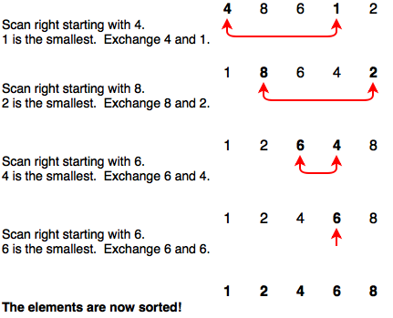The selection sort works as follows:
Search the entire array to find the smallest value. Exchange that value with the value in the first position of the array. Next, scan the rest of the array (all but the first element) to find the smallest value, and then exchange it with the value in the second element of the array. Next, scan the rest of the array (all but the first two elements) to find the smallest value, and then exchange it with the value in the third element of the array. Continue this process for each element in the array. The number of passes required is one less than the length of the array. When the process is complete, the array will be sorted.Using the BubbleSort class as a model, create a SelectionSort class and a SelectionSortTest class to demonstrate it.
Once you have your selection sort algorithm working, time it against RANDOM, ASCENDING, and DESCENDING data sets of 100,000 elements. Again, make sure you are generating a broad range of random integers in your constructor using the statement: data[ i ] = generator.nextInt(); Record your results and compare them with your bubble sort v3.0 results from Q1. Explain which sort is best given random, ascending, or descending data sets. If there are any significant performance differences, hypothesize why this might be so.