Big O Notation
There are often several algorithms to choose from to solve the same problem. As we saw last time, there are many factors that go into choosing the best algorithm for a given situation. One tool that computer scientists use to compare the performance of different algorithms is called Big O notation – the “O” stands for “order of complexity”. The best way to understand Big O is through examples.
O(1): “Order 1”
Imagine that I have already created an integer array called myArray. Consider the following code:
|
1 2 3 |
// O(1) -- "Order 1" myArray[2] = 99; System.out.println(myArray.length); |
Regardless of the number of elements in the array, this sequence of statements will always require the same amount of time to execute. When code executes in a constant amount of time, it is referred to as “Order 1”, or O(1) in Big O notation. If we were to graph this performance, it would be a horizontal line.
O(n): “Order n”
Consider again the linear search algorithm:
|
1 2 3 4 5 6 7 |
// O(n) -- "Order n" for ( int index = 0; index < data.length; index++ ) { if ( data[ index ] == searchKey ) { return index; // return index of integer } } return -1; // integer was not found |
Assuming the data array is not empty, this loop may iterate anywhere from 1 time (if the searchkey is found in the first element of the data array) to data.length times (if the searchkey is not found at all). But on average, if there are n elements in the array, we can expect to compare ½n elements to find the searchKey.
From your knowledge of math, you know that the graph of ½n is linear. Even if we ignore the coefficient of ½ the nature of the graph would still be linear, only the slope would change. Because of this fact, we can safely drop the coefficient, and thus refer to its performance as “Order n”, or O(n).
O(n2): “Order n-squared”
Inspect the following code:
|
1 2 3 4 5 6 |
// O(n^2) -- "Order n-squared" for (j = 0; j < n; j++) { for (k = 0; k < n; k++) { ...inner loop code repeats n x n times... } } |
Now things get more interesting! Here we go through the outer loop n times and for each of these iterations we go through the inner loop n times. Overall, the code in the inner loop is executed n x n, or n2 times. We call this “Order n2”, or O(n2).
Here’s another example:
|
1 2 3 4 5 |
for (j = 0; j < n; j++) { for (k = 0; k < (n + 50); k++) { ...inner loop code repeats n x (n + 50) times... } } |
In this case, the code in the inner loop will repeat n x (n + 50) times, or n2+50n. We know that this is a quadratic graph. Even if we discard the + 50n part and keep only the term with the highest exponent (n2) the nature of the graph does not change. Therefore the Big O for this code is O(n2).
Let’s look at one more:
|
1 2 3 4 5 |
for (j = 0; j < n ; j++) { for (k = 0; k < (n * 50); k++) { ...inner loop code repeats n x (n x 50) times... } } |
Here the inner loop code will repeat n x (50 x n) times, or 50n2 times. Again we have a quadratic. Even if we ignore the coefficient of 50, the nature of the graph does not change. Therefore the Big O for this code is again O(n2).
O(n3): “Order n-cubed”
Let’s say we analyze some code and obtain the expression: (3/5)n3+15n2 + (1/2)n + 5. At this point, just by looking at this expression we can imagine that the code includes 1 triple-nested loop (i.e., n3), 1 double-nested loop (i.e., n2), 1 single loop (i.e., n), and some code with constant run-time.
To determine the Big O notation for this expression we can safely ignore any coefficients and constants to give us: n3+n2 + n. Next, we can eliminate all terms but the one with the highest exponent leaving us with n3, thus the Big O notation is simply O(n3). Easy eh? If you’ve struggled with graphing mathematical functions in school, simplifying with Big O can be very satisfying!
O(log n): “Order log-n”
Let’s think about the binary search algorithm again. Binary search is so efficient because it continuously cuts the amount of data to be searched in half with each comparison. The best case would be that the search key is found in the middle of the data on the first comparison. The worst case occurs if the search key is not present in the data at all, in which case log2n comparisons would be needed to confirm this. But on average, we would expect to find the search key after ½ log2n comparisons.
It’s clear that the nature of the algorithm is logarithmic, so we can safely drop the base and ignore the ½ giving O(log n).
O(nlog n): “Order nlog-n”
One final example:
|
1 2 3 4 5 |
for (j = 0; j < n; j+=5) { for (k =1; k < n; k*=3) { ...inner loop code repeats 1/5n x log3n times... } } |
Here the outer loop will repeat (1/5)n times because we are incrementing the loop control variable j by 5 after each iteration. The inner loop control variable k is tripled after each iteration, therefore the inner loop will repeat log3n times. Putting these together gives us the expression (1/5)n x log3n. As is the custom with Big O, we can safely drop the coefficient of 1/5. We can also drop the base 3 on the log since this does not change the nature of the graph – it’s still logarithmic. This leaves us with O(nlog n).
Comparsion of Growth Functions
As I said that the start, Big O is a useful tool for comparing the theoretical efficiency of different algorithms. To really appreciate this, let’s plot the graphs of O(n), O(n2), O(n3), O(log n), and O(nlog n) together.
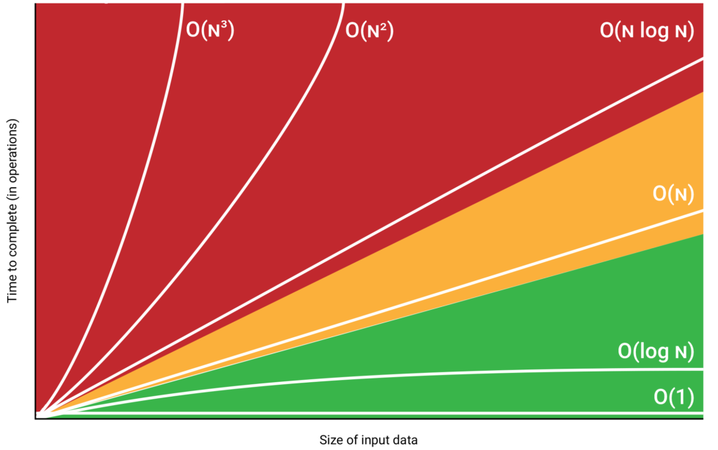
From the graph it’s obvious that O(n3), O(n2), and O(nlog n) algorithms should be avoided if the input size is large – the processing time increases exponentially! Conversely, O(log n) is clearly superior for large data sets – as n increases, processing time increases at a much slower rate.
O(n) algorithms can fall somewhere in the middle. If there is a large coefficient on n the linear performance graph would have a steeper slope (and the opposite is also true).
To help drive the point home, below is a variety of input sizes (n) processed by algorithms with different Big O growth rates.
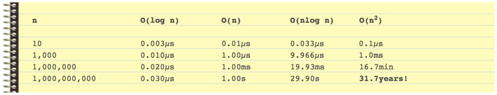
Choosing the right algorithm can make a huge difference, so choose wisely!
Limitations of Big O
So, can we conclude that O(n2) algorithms should be avoided at all costs?
No! If you look carefully at the graphs above you’ll notice that when the number of items (n) being processed is small, there is very little performance difference between them. For example, if you only need to search 10 or fewer elements, it would make more sense to code a linear search O(n) rather than a binary search O(log n). Why use a power tool when a simple hand tool will suffice?
It’s only when the number of items (n) becomes large that Big O becomes a more useful analysis tool. But even this can be misleading! Big O is concerned with the average case, and usually assumes randomly ordered data. In the real world, data may be sorted in ascending, descending, or nearly sorted order and this can have a huge impact on algorithm efficiency.
The bottom line is that while Big O provides a performance guideline, the only real way to know for sure is to actually test different algorithms with a variety of data sets. Even if two algorithms have the same Big O, their performances can still differ significantly.
You Try!
- Figure out the Big O notation for the following 5 algorithms:
12345678910111213141516171819202122232425262728293031323334// Algorithm 1for (j = 0; j < n + 5; j++) {...some code...}// Algorithm 2for (j = 0; j < n - 5; j++) {for (k = 0; k < 7; k++) {...some code...}}// Algorithm 3for (j = 2; j < n + 5; j*=7) {...some code...}// Algorithm 4for (j = 0 ;j < n - 5; j++) {for (k = 0; k < n; k++) {...some code...}}// Algorithm 5for (j = 0; j < n; j+=2) {for (k = 1; k < n; k = k * 8) {...some code...}} - In the algorithms above, assuming n is a large number, order the algorithms from least to most efficient based on their Big O notations.